February 2nd, 2022
Hyperparameter Optimization – What, Why and How?
Introduction
A mathematical model can describe a natural phenomenon when provided with an appropriate set of data. Such a model always contains some parameters which are to be determined for a given set of data points. For example, the famous linear least squares model as shown in Figure 1 is built with two parameters – the slope (W1) and the intercept (W0).
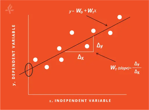
As can be seen from the figure, varying the slope, the intercept or the both can determine if the line represents the data well enough. Therefore, it is crucial to obtain the best values of these parameters in order to have a robust model. Given a dataset, these two parameters can be obtained such that the model predicts with a reasonable accuracy as to how far a new data point is located from the line. This process of estimating the best parameters for a dataset is called training the model. During training, the model parameters are estimated by optimizing a cost function and using the available dataset. A similar approach is also followed while developing a robust Machine Learning (ML) or a Deep Learning (DL) model for a given problem.
There is always a historical dataset and a learning algorithm to develop the ML model. Each of the learning algorithms can have a large set of parameters which are called hyperparameters. At this juncture, it is necessary to understand the difference between the model parameters and the hyperparameters. In Figure 2, it is shown that the model parameters and the hyperparameters are two disjoint sets having no parameters in common. The parameters W0, W1, W2,… etc. are part of the model, whereas learning rate, optimizer choice, batch size, n_neighbors, kernel etc. are part of the learning algorithm and has nothing to do with the model.
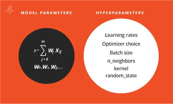
The model parameters are internal to the model and are estimated during training based on the historical dataset available whereas the hyperparameters are not part of the model and are predefined before the training. The model parameters, and not the hyperparameters, are saved and used during predictions. In the case of linear least squares fitting, the slope and the intercept are the model parameters.
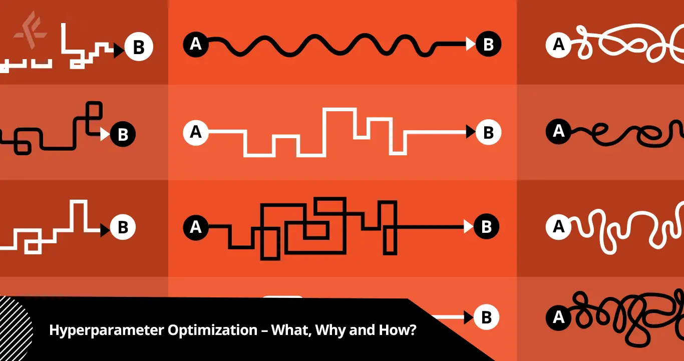
It is to be noted that choosing the appropriate subset of hyperparameters with the best values is important as these hyperparameters will affect the speed and accuracy of the training. Depending upon the system or the problem at hand, the number of hyperparameters required for training is going to be different. Thus, choosing the right set of hyperparameters is a rather tricky and challenging task. These parameters form an n-dimensional search space where each dimension is one such parameter.
A point on this search space is then a specific combination of values of these parameters. The more the number of parameters, the larger the search space, and the problem of finding the best values turns more complex.
Optimization Techniques
n*=arg f(η) (1)
Optimization of hyperparameters is always associated with an objective function (f(η) as in equation (1)) that needs to be either minimized or maximized depending upon the evaluating metric defined for the problem at hand.
This optimization is then to obtain the set of hyperparameters that yields the optimum value to this objective function.
In equation (1), * is the set of hyperparameters that yields the optimum value of the objective function. One can perform the optimization in a brute force way. However, such an approach can be cumbersome. For example, if one needs to optimize three parameters of a learning algorithm and to start with, let us say there are two values of each parameter to be tried.
This leads to eight possible combinations of values. Now imagine we have ten parameters, and we want to try out five possible values for each of them. Already turns out to be a humongous task as one has to run the learning algorithm for each of these combinations. As saviors, there are optimization algorithms that can automate this whole process of parameter search and give us with the best possible combination.
One of the popular optimization methods is called ‘grid search’. In a grid search algorithm, the parameter search space is divided into grid points (combinations of values) and at each grid point the learning algorithm is run, the appropriate metric (accuracy, loss etc.) is evaluated, and finally, the best possible combination of the hyperparameter values is obtained. On the other hand, in the random search method, the parameter values are sampled randomly from the defined bounded values of these parameters.
Random search method can be useful when one cannot intuitively guess the initial values of the parameters. Notably, these two techniques are inefficient as they do not take in to account the past results for evaluating the next hyperparameters.
Bayesian optimization is another commonly used method that takes care of the previous results while evaluating the next hyperparameters and this method is useful when the objective function is complex and computationally expensive to calculate. The Bayesian method uses the Bayes theorem to direct the search for the maximum or the minimum of the objective function. In fact, there are several such optimization algorithms that are available in the literature.
Optuna and Automated Optimization
In an ML model development process, the implementation of automated hyperparameter tuning is of utmost necessity as it reduces the manual effort to get the best possible combination of values of the chosen hyperparameters.
Optuna is an open-source Python library that can be used to automate hyperparameter tuning for any ML problem. Optuna can be used with many ML frameworks such as TensorFlow, PyTorch, LightGBM, and scikit-learn. Among various features, Optuna uses a pruning mechanism to save time in the whole optimization process. As we mentioned above, the hyperparameter optimization can be time consuming if we choose a large number of parameters in the search space. In the pruning mechanism, any unreasonable or unpromising trials are terminated at the early stage of the training saving time and resources.
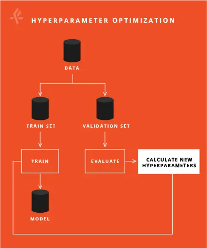
A typical hyperparameter tuning process is shown in Figure 3. The baseline model is trained with the train dataset and then the model is evaluated with the validation dataset. The evaluation of the model is done based on a predefined metric such as accuracy or average F1 score.
Hyperparameter tuning in our ML pipeline is done as follows. To start with, the baseline model is trained and evaluated with the training and the validation datasets, respectively. Based on the performance on the validation set, new hyperparameters are calculated and used for next training iteration. This process is repeated until the best model is obtained.